# load libraries
library(isoorbi) # for Orbitrap functions
library(dplyr) # for data wrangling
library(ggplot2) # for data visualization
Data
Load raw file(s)
# read raw files including 1 spectrum
raw_files <-
  c("ac5.RAW", "ac6.RAW", "s3744.RAW") |>
  orbi_get_example_files() |>
  orbi_read_raw(include_spectra = 100) |>
  orbi_aggregate_raw()
# quick glance at the spectra (m/z range 96 to 102)
raw_files |> orbi_plot_spectra(96, 102)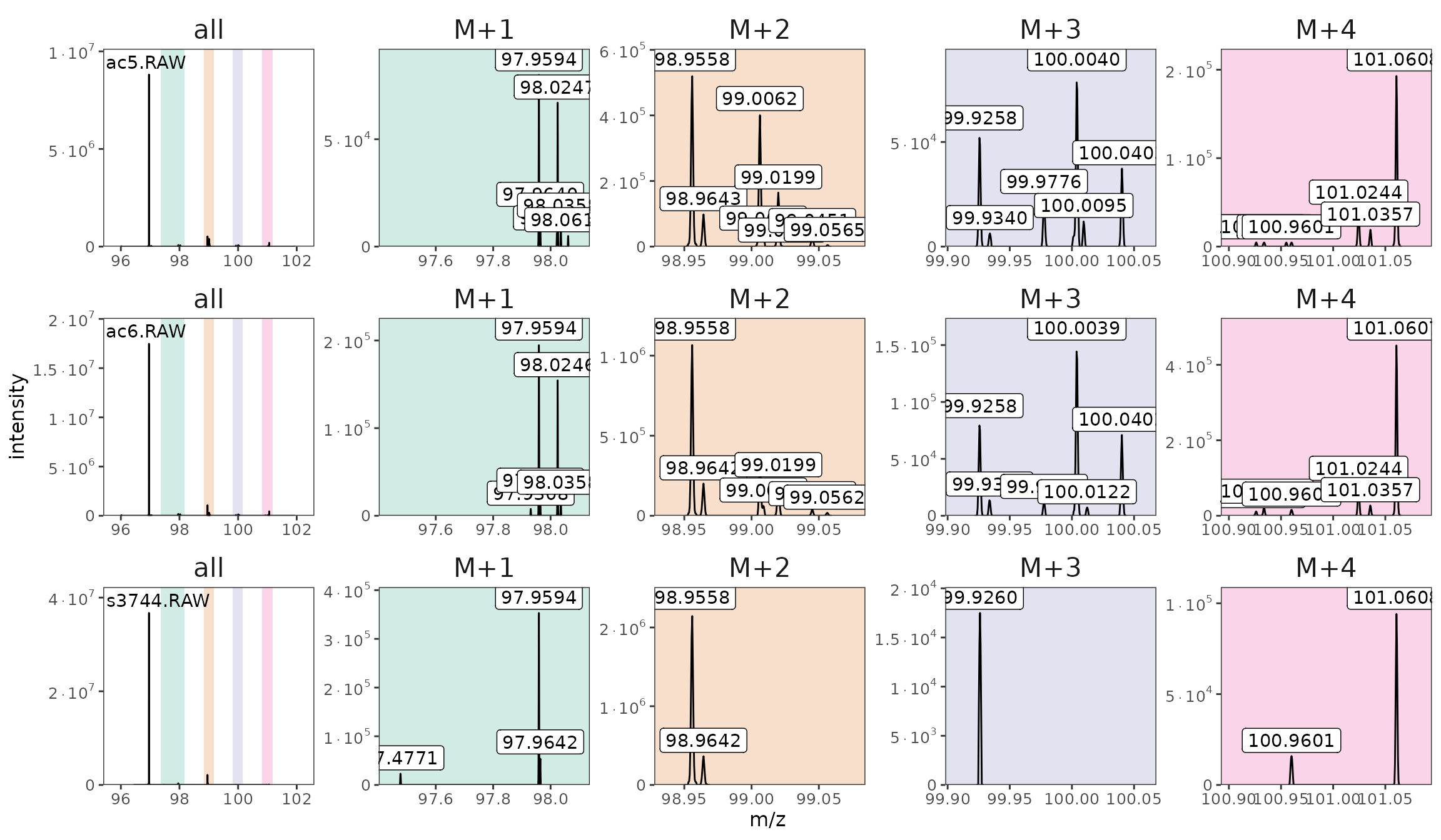
One spectrum from each file with the M+x regions highlighted.
Identify isotopocules
# identify sulfate isotopocules
# could come from a tsv, csv, or xlsx spreadsheet instead
isotopocules <- tibble(
  compound = "HSO4-",
  isotopocule = c(
    "M0", "33S", "17O", "34S", "18O",
    # also look for a few clumped isotopocules
    "33S18O", "34S17O", "36S", "18O18O"),
  mass = c(
    96.96000, 97.95940, 97.96420, 98.95580, 98.96430,
    99.9632, 99.9590, 100.9551, 100.968046)
)

# identify
raw_files_w_isotopocules <- raw_files |>
  orbi_identify_isotopocules(isotopocules) |>
  # disregard unidentified isotopocules but keep missing
  orbi_filter_isotopocules(keep_missing = TRUE) |>
  # check for minor peaks that are in the same mass tolerance
  # window of an isotopocule
  orbi_flag_satellite_peaks()
# plot again now with the isotopocules identified
raw_files_w_isotopocules |> orbi_plot_spectra(96, 102)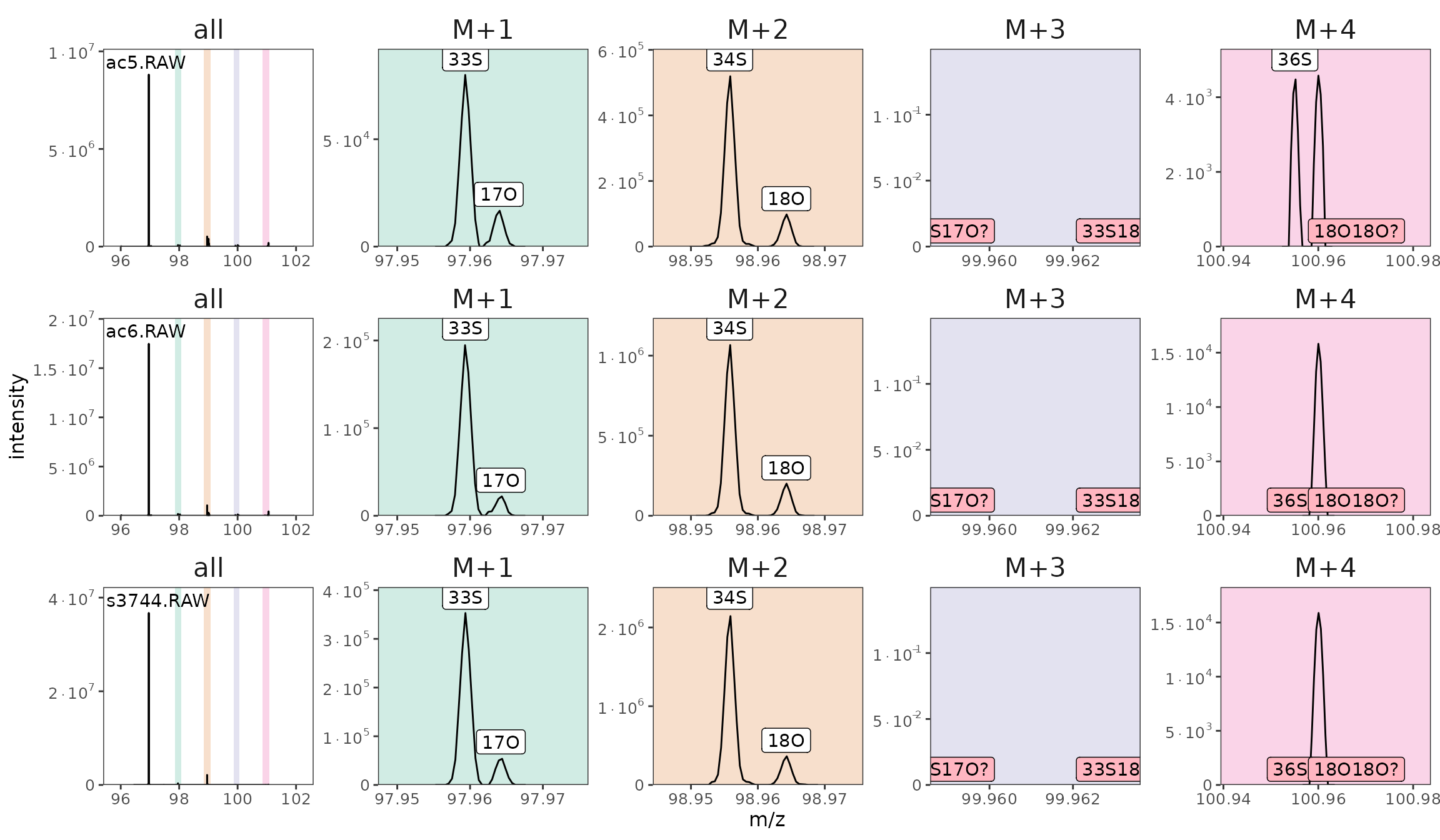
Spectra with identified isotopocules (missing ones highlighted in pink).
# check coverage (as suggested during isotopocule identifiation)
raw_files_w_isotopocules |> orbi_plot_isotopocule_coverage()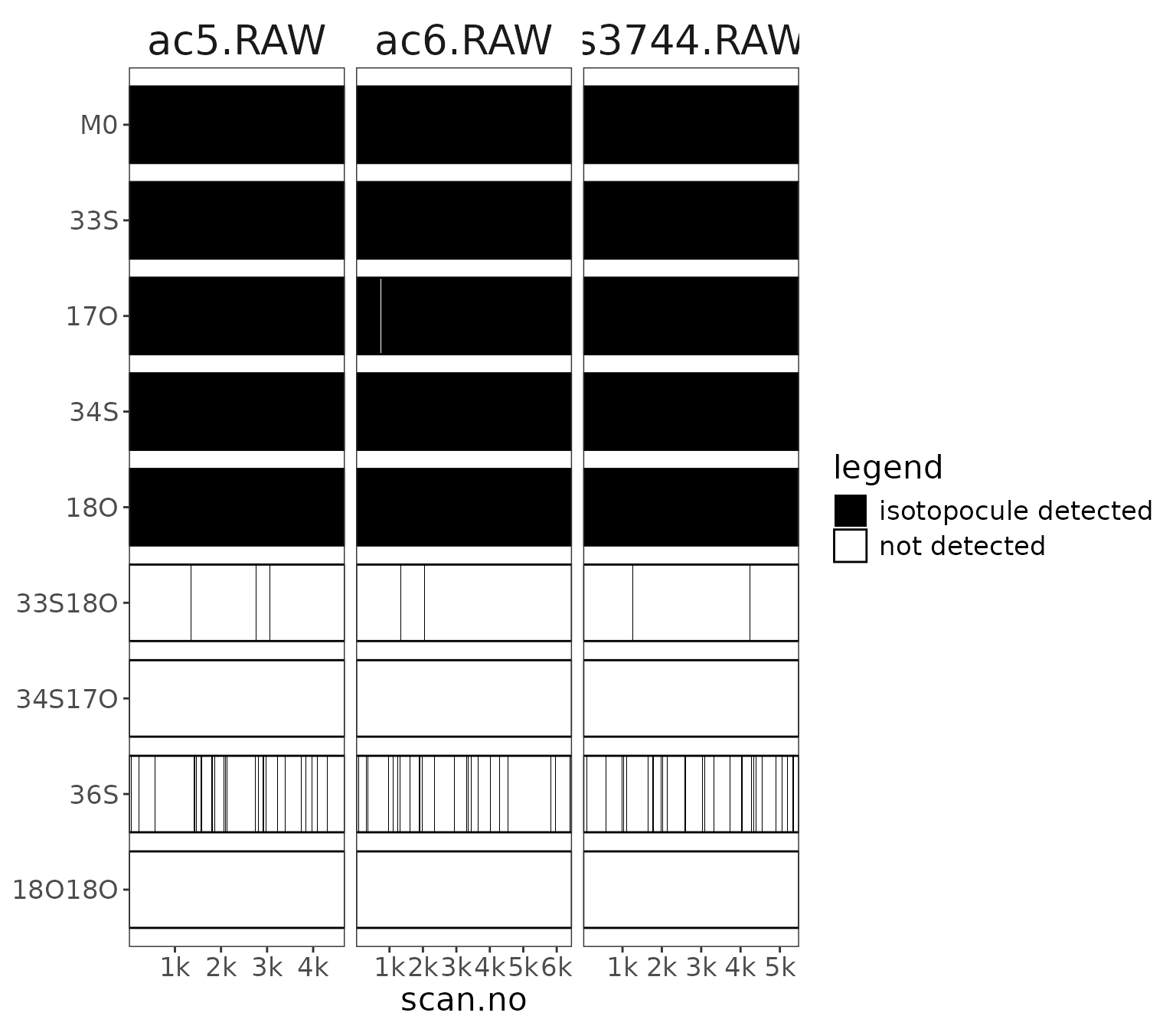
isotopocule coverage in each file across the scans.
Processing
It’s clear from the plots above that we don’t have good coverage for the clumped isotopocules and 36S (i.e. they are missing from some/many scans). We won’t work with these further anyways but it’s a good visual example of how much harder these are to detect.
# Preprocess data (this is exactly the same as with an isox file)
data <-
  raw_files_w_isotopocules |>
  # focus on the main single substitutions
  orbi_filter_isotopocules(c("M0", "33S", "17O", "34S", "18O")) |>
  # double check the remainng isotopcoules
  orbi_flag_weak_isotopocules(min_percent = 99) |>
  # flags outlying scans that have more than 2 times or less than
  # 1/2 times the average number of ions in the Orbitrap analyzer
  orbi_flag_outliers(agc_fold_cutoff = 2) |>
  # sets one isotopocule in the dataset as the base peak
  # (denominator) for ratio calculation
orbi_define_basepeak(basepeak_def = "M0") Let’s take a look at the AGC cutoff flagged samples
# in terms of scans
orbi_plot_raw_data(data, y = tic * it.ms, y_scale = "log")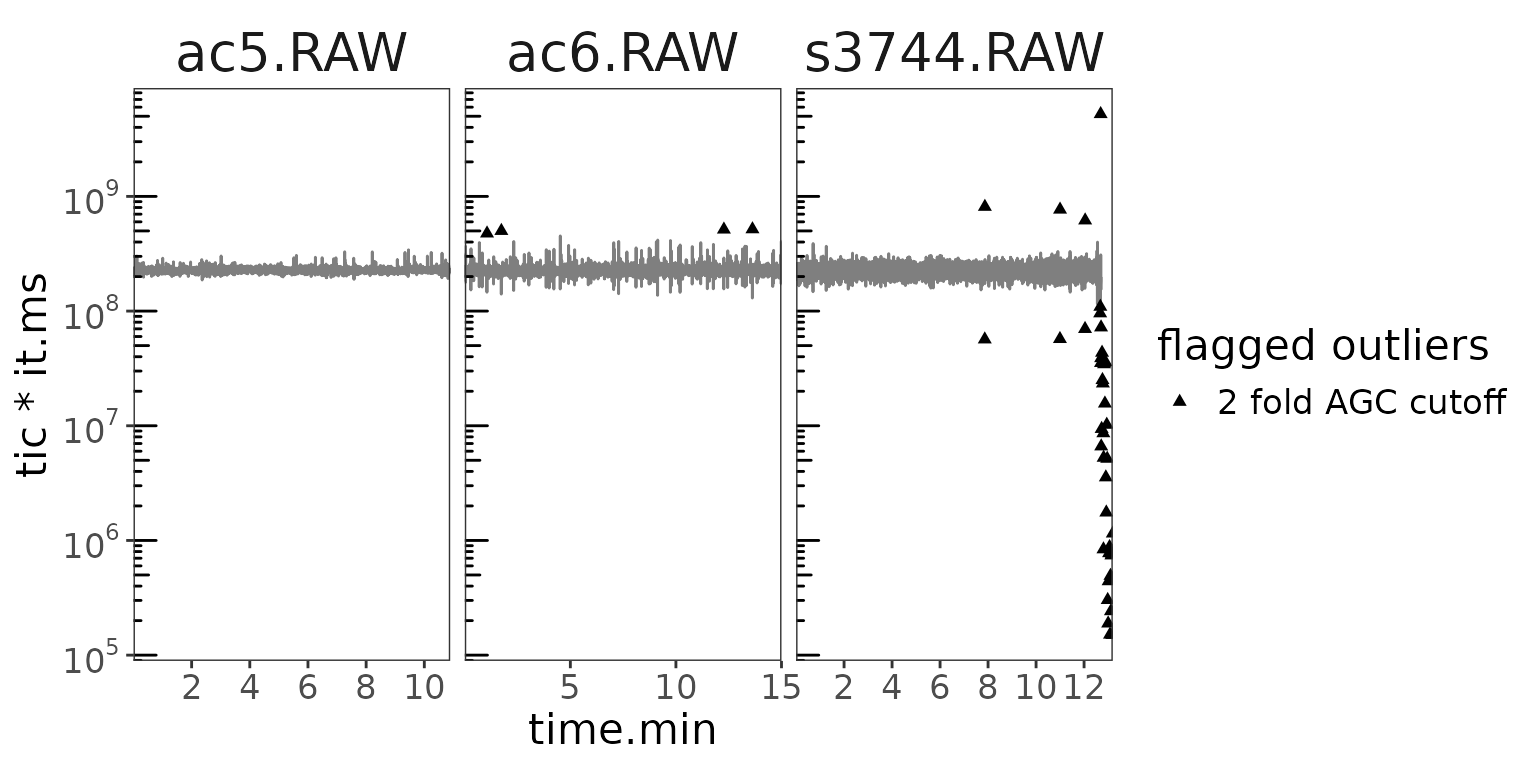
Estimated ions in the analyzer
# and in terms of the ions
orbi_plot_raw_data(data, y = ions.incremental, y_scale = "log")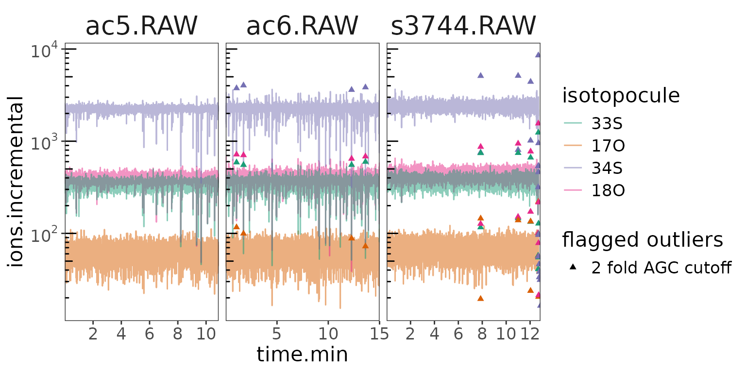
Isotopocules ions
Seems like the issue is mostly towards the end of the s3744 analysis. What about the resulting ratios?
data |> orbi_plot_raw_data(y = ratio) 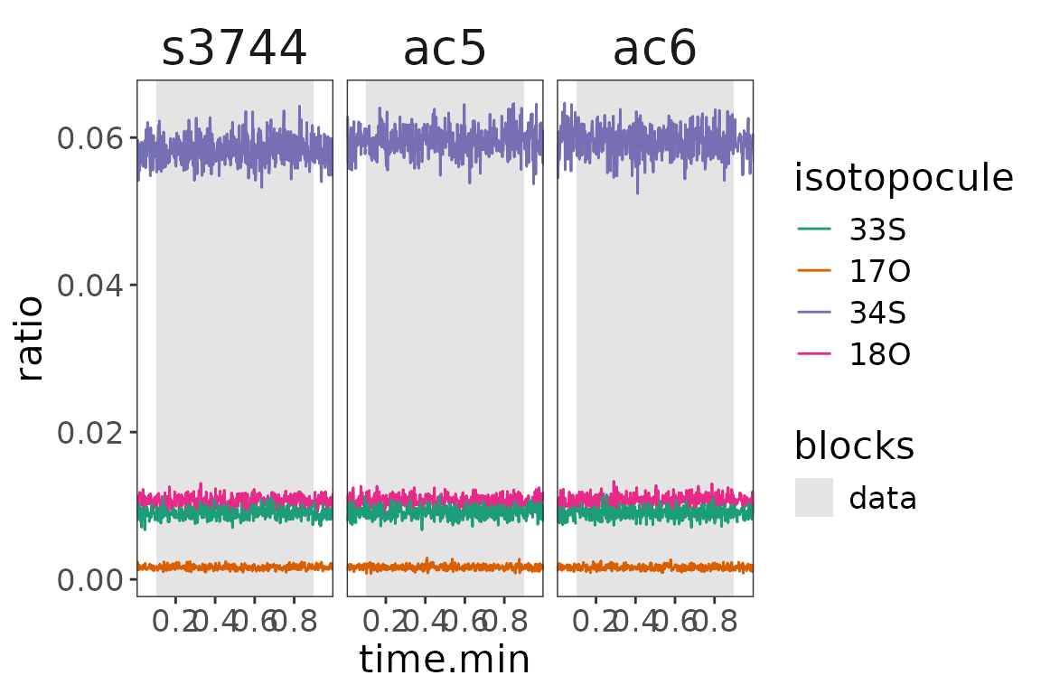
Isotopocule ratios vs M0
The ratios suggest that there really is an issue at the end of the s3744 run. Having flagged these outliers, they will automatically not be included in the summary calculation of the resulting ratios.
Summary
# summarize the ratio summaries
data_summary <-
  data |>
  orbi_summarize_results(ratio_method = "sum")
# data
data_summary |>
orbi_get_data(summary = c("compound", "isotopocule", starts_with("ratio")))# A tibble: 12 × 7
uidx filename compound isotopocule ratio ratio_relative_sem_p…¹ ratio_sem
<int> <chr> <fct> <fct> <dbl> <dbl> <dbl>
1 1 ac5.RAW HSO4- 33S 0.00903 1.18 1.06e-5
2 1 ac5.RAW HSO4- 17O 0.00165 2.92 4.81e-6
3 1 ac5.RAW HSO4- 34S 0.0599 0.459 2.75e-5
4 1 ac5.RAW HSO4- 18O 0.0107 1.06 1.13e-5
5 2 ac6.RAW HSO4- 33S 0.00902 0.99 8.92e-6
6 2 ac6.RAW HSO4- 17O 0.00164 2.47 4.05e-6
7 2 ac6.RAW HSO4- 34S 0.0595 0.4 2.38e-5
8 2 ac6.RAW HSO4- 18O 0.0106 0.911 9.67e-6
9 3 s3744.RAW HSO4- 33S 0.00894 1.01 9.07e-6
10 3 s3744.RAW HSO4- 17O 0.00164 2.58 4.23e-6
11 3 s3744.RAW HSO4- 34S 0.0584 0.414 2.42e-5
12 3 s3744.RAW HSO4- 18O 0.0106 0.944 1.00e-5
# ℹ abbreviated name: ¹ratio_relative_sem_permil
# export file info and summary to excel
data_summary |> orbi_export_data_to_excel(
  file = "output.xlsx",
  include = c("file_info", "summary")
)
fig <-
  data_summary |>
  # get out all summary data
  orbi_get_data(summary = everything()) |>
  # generate a custom label for the data panels
  mutate(panel = glue::glue("ratio\n{isotopocule} / {basepeak}")) |>
  # plot
  ggplot() +
  aes(
    x = filename,
    y = ratio, ymin = ratio - ratio_sem, ymax = ratio + ratio_sem,
    color = filename, shape = filename
  ) +
  geom_pointrange(size = 1) +
  scale_color_brewer(palette = "Dark2") +
  scale_y_continuous(breaks = scales::pretty_breaks(5)) +
  facet_grid(panel ~ ., scales = "free_y", switch = "y") +
  # styling
  theme_bw() +
  theme(
    text = element_text(size = 16),
    panel.grid = element_blank(),
    strip.text.y.left = element_text(angle = 0),
    strip.placement = "outside",
    strip.background = element_blank()
  ) +
  labs(y = NULL, x = NULL)
fig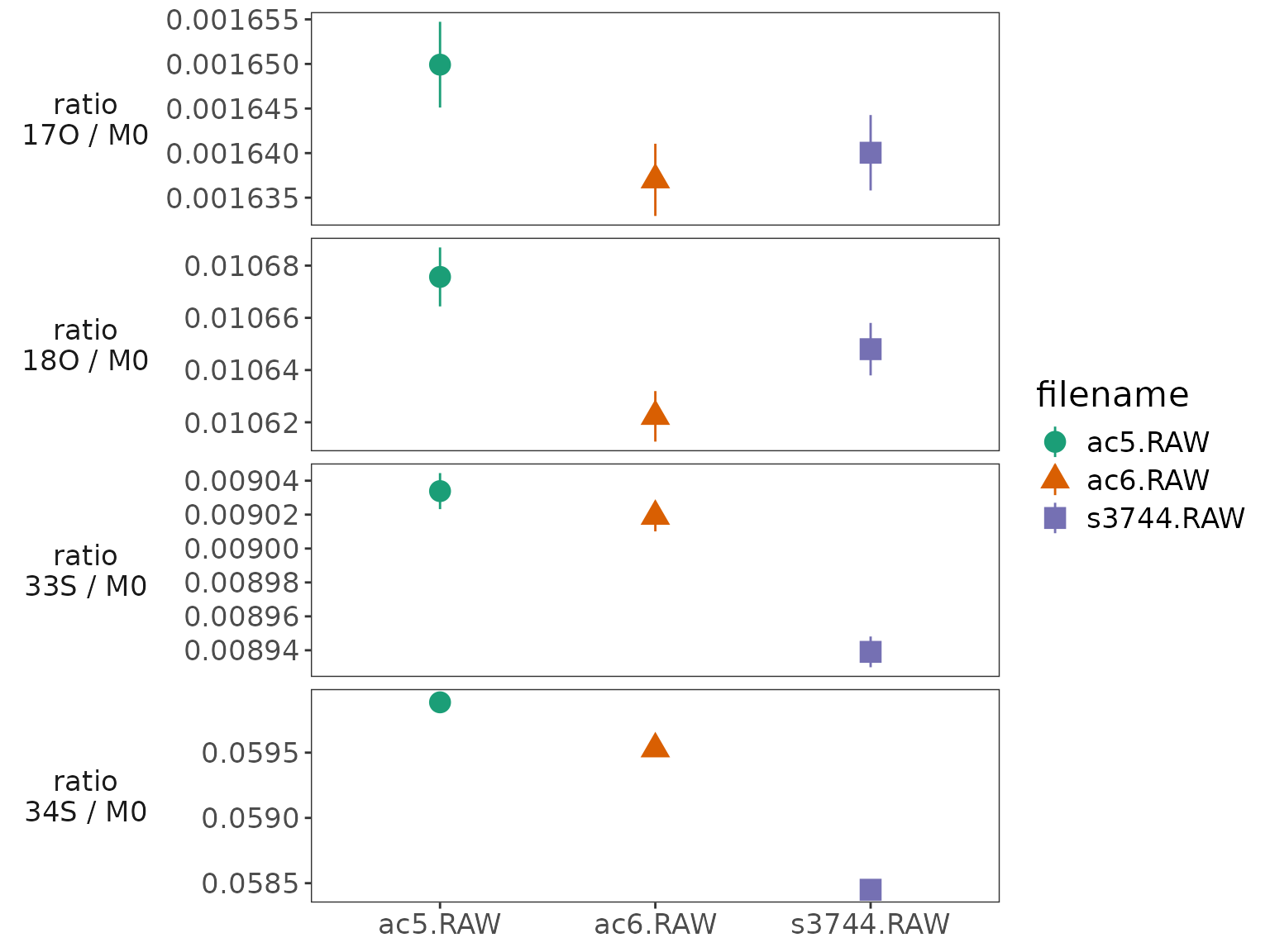
Isotopocule ratios summary