This is a minimal example for processing .raw data files from a dual inlet experiment
# libraries
library(isoorbi) #load isoorbi R package
library(forcats) #better ordering of factor variables in plots
library(dplyr) # for mutating data frames
library(ggplot2) # for data visualization
Load raw file(s)
# Read test data .raw file
raw_file <- orbi_get_example_files("dual_inlet.raw")

data_all <-
  raw_file |>
  orbi_read_raw(include_spectra = c(10, 100)) |>
  orbi_aggregate_raw()
# identify nitrate isotopocules
# could come from a tsv, csv, or xlsx spreadsheet instead
isotopocules <- tibble(
  compound = "nitrate",
  isotopocule = c("M0", "15N", "17O", "18O"),
  mass = c(61.9878, 62.9850, 62.9922, 63.9922)
)
data_all <- data_all |>
  orbi_identify_isotopocules(isotopocules) |>
  # disregard unidentified and missing isotopocules
  orbi_filter_isotopocules()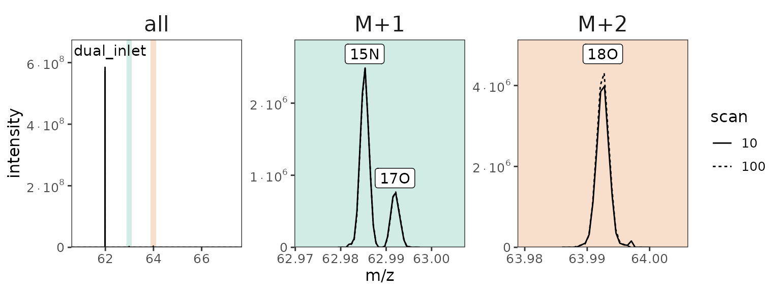
Preprocess data
# Preprocess data (this is exactly the same as with an isox file)
df <-
  data_all |>
  # check for issues
  # removes minor peaks that are in the same mass tolerance window
  # of an isotopocule
  orbi_flag_satellite_peaks() |>
  # flag signals of isotopocules that were not detected
  # in all scans
  orbi_flag_weak_isotopocules(min_percent = 100) |>
  # flags outlying scans that have more than 2 times or less than
  # 1/2 times the average number of ions in the Orbitrap analyzer;
  # another method: agc_window (see function documentation for more details)
  orbi_flag_outliers(agc_fold_cutoff = 2) |>
  # sets one isotopocule in the dataset as the base peak
  # (denominator) for ratio calculation
orbi_define_basepeak(basepeak_def = "M0") No satellite peaks, no weak isotopocules, a few AGC fold outliers:
df |> orbi_plot_raw_data(y = tic * it.ms, y_scale = "log")
Define dual inlet blocks
# define blocks
df_w_blocks <-
  df |>
  # general definition
  orbi_define_blocks_for_dual_inlet(
    # the reference block is 10 min long
    ref_block_time.min = 10,
    # the sample block is 10 min long
    sample_block_time.min = 10,
    # there is 5 min of data before the reference block starts,
    # to stabilize spray conditions
    startup_time.min = 5,
    # it takes 2 min to make sure the right solution is measured
    # after switching the valve
    change_over_time.min = 2,
    sample_block_name = "sample",
    ref_block_name = "reference"
  ) |>
  # fine adjustments
  # the 1st reference block is shorter by 2 min, cut from the start
  orbi_adjust_block(block = 1, shift_start_time.min = 2) |>
  # the start and end of the 2nd reference block are manually set
  orbi_adjust_block(block = 4, set_start_time.min = 38, set_end_time.min = 44)
# get blocks info
blocks_info <- df_w_blocks |> orbi_get_blocks_info()
blocks_info |> knitr::kable()| uidx | filename | data_group | block | sample_name | data_type | segment | start_scan.no | end_scan.no | start_time.min | end_time.min |
|---|---|---|---|---|---|---|---|---|---|---|
| 1 | dual_inlet | 1 | 0 | reference | startup | NA | 1 | 822 | 0.0069267 | 4.996783 |
| 1 | dual_inlet | 2 | 1 | reference | unused | NA | 823 | 1152 | 5.0028499 | 7.002534 |
| 1 | dual_inlet | 3 | 1 | reference | data | NA | 1153 | 2467 | 7.0086023 | 14.994198 |
| 1 | dual_inlet | 4 | 2 | sample | changeover | NA | 2468 | 2796 | 15.0002893 | 16.996492 |
| 1 | dual_inlet | 5 | 2 | sample | data | NA | 2797 | 4112 | 17.0025578 | 24.994222 |
| 1 | dual_inlet | 6 | 3 | reference | changeover | NA | 4113 | 4441 | 25.0005399 | 26.997343 |
| 1 | dual_inlet | 7 | 3 | reference | data | NA | 4442 | 5757 | 27.0034184 | 34.995687 |
| 1 | dual_inlet | 8 | 4 | sample | changeover | NA | 5758 | 6086 | 35.0019892 | 36.998449 |
| 1 | dual_inlet | 9 | 4 | sample | unused | NA | 6087 | 6250 | 37.0045150 | 37.994845 |
| 1 | dual_inlet | 10 | 4 | sample | data | NA | 6251 | 7238 | 38.0009123 | 43.999949 |
| 1 | dual_inlet | 11 | 4 | sample | unused | NA | 7239 | 7402 | 44.0060263 | 44.996372 |
| 1 | dual_inlet | 12 | 5 | reference | changeover | NA | 7403 | 7730 | 45.0026717 | 46.994070 |
| 1 | dual_inlet | 13 | 5 | reference | data | NA | 7731 | 9047 | 47.0001525 | 54.996822 |
| 1 | dual_inlet | 14 | 6 | sample | changeover | NA | 9048 | 9376 | 55.0031201 | 56.999885 |
| 1 | dual_inlet | 15 | 6 | sample | data | NA | 9377 | 10692 | 57.0059518 | 64.997181 |
| 1 | dual_inlet | 16 | 7 | reference | changeover | NA | 10693 | 11020 | 65.0035025 | 66.994101 |
| 1 | dual_inlet | 17 | 7 | reference | data | NA | 11021 | 12337 | 67.0001943 | 74.997220 |
| 1 | dual_inlet | 18 | 8 | sample | changeover | NA | 12338 | 12338 | 75.0035170 | 75.003517 |
Raw data plots
Plot 1: default block highlights + outliers
# total ions per scan
df_w_blocks |> orbi_plot_raw_data(y = intensity, y_scale = "linear")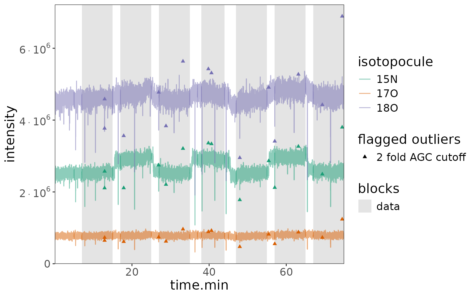
# isotopocule ratios - you can see that even the AGC outliers
# still create decent ratios
df_w_blocks |>  orbi_plot_raw_data(y = ratio)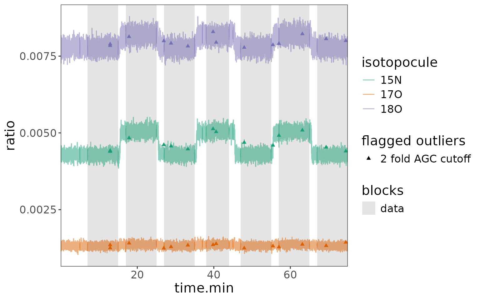
Plot 2: highlight blocks in data + no outliers
df_w_blocks |>
  orbi_plot_raw_data(
    isotopocules = "15N",
    y = ratio,
    color = NULL,
    add_all_blocks = TRUE,
    show_outliers = FALSE
  ) +
  # add other ggplot elements, e.g. more specific axis labels
  labs(x = "time [min]", y = "15N/M0 ratio")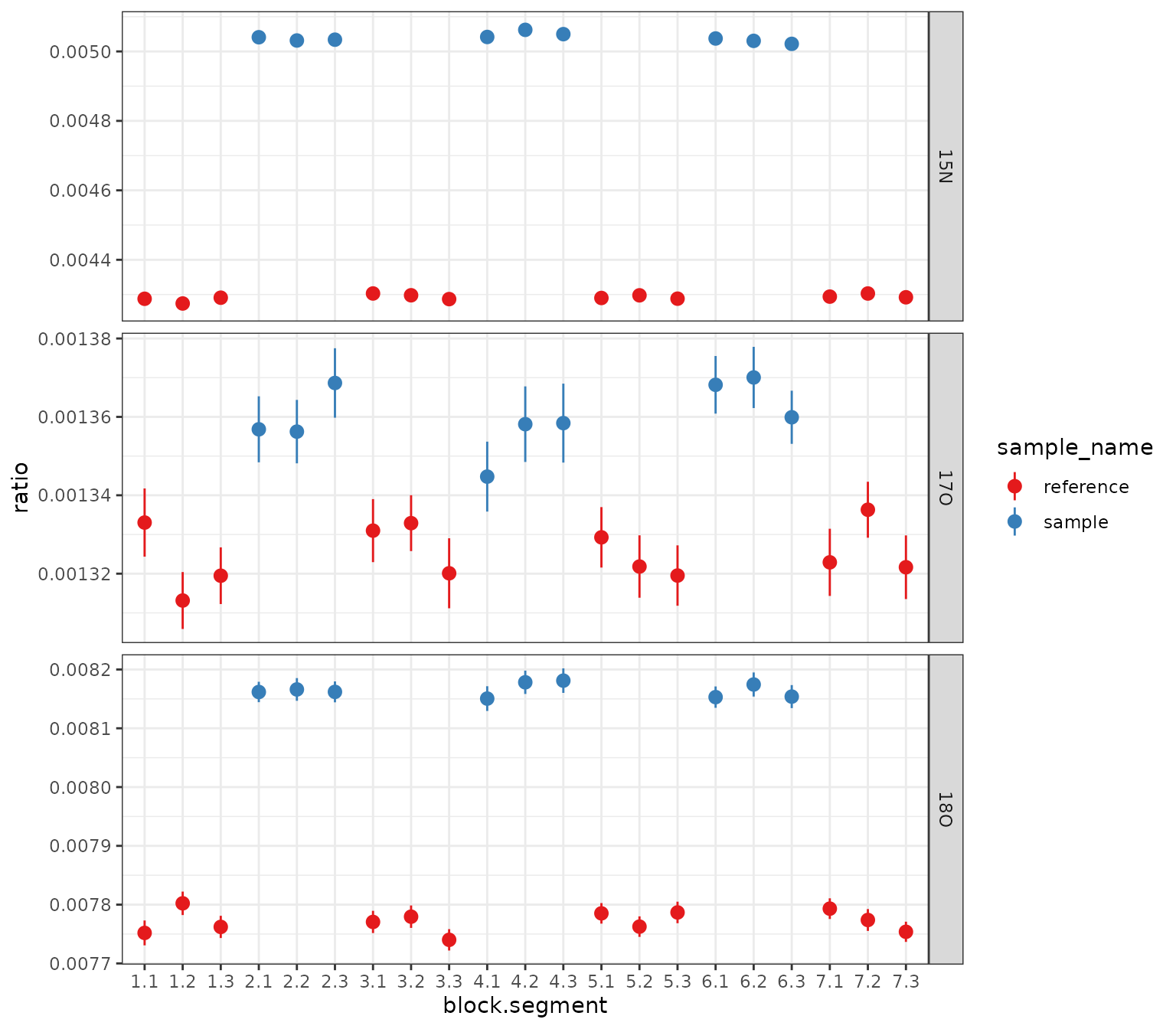
Plot 3: highlight sample blocks on top
df_w_blocks |>
  orbi_plot_raw_data(
    isotopocules = "15N",
    y = ratio,
    add_all_blocks = TRUE,
    show_outliers = FALSE,
    color = factor(block)
  ) +
  labs(x = "time [min]", y = "15N/M0 ratio", color = "block #")
Data summaries
# calculate summary
df_w_summary <-
  df_w_blocks |>
  # segment (optional)
  orbi_segment_blocks(into_segments = 3) |>
  # calculate results, including for the unused parts of the data blocks
  orbi_summarize_results(
    ratio_method = "sum",
    include_unused_data = TRUE
  )
# export file info and summary to excel
df_w_summary |> orbi_export_data_to_excel(
  file = "output.xlsx",
  include = c("file_info", "summary")
)Plot 1: ratios summary by block and segment
# get out the summary and plot all isotopocules using a ggplot from scratch
df_w_summary |>
  orbi_get_data(summary = everything()) |>
  filter(data_type == "data") |>
  mutate(block_seg = sprintf("%s.%s", block, segment) |> fct_inorder()) |>
  # data
  ggplot() +
  aes(
    x = block_seg,
    y = ratio, ymin = ratio - ratio_sem, ymax = ratio + ratio_sem,
    color = sample_name
  ) +
  geom_pointrange() +
  facet_grid(isotopocule ~ ., scales = "free_y") +
  # scales
  scale_color_brewer(palette = "Set1") +
  theme_bw() +
  labs(x = "block.segment", y = "ratio")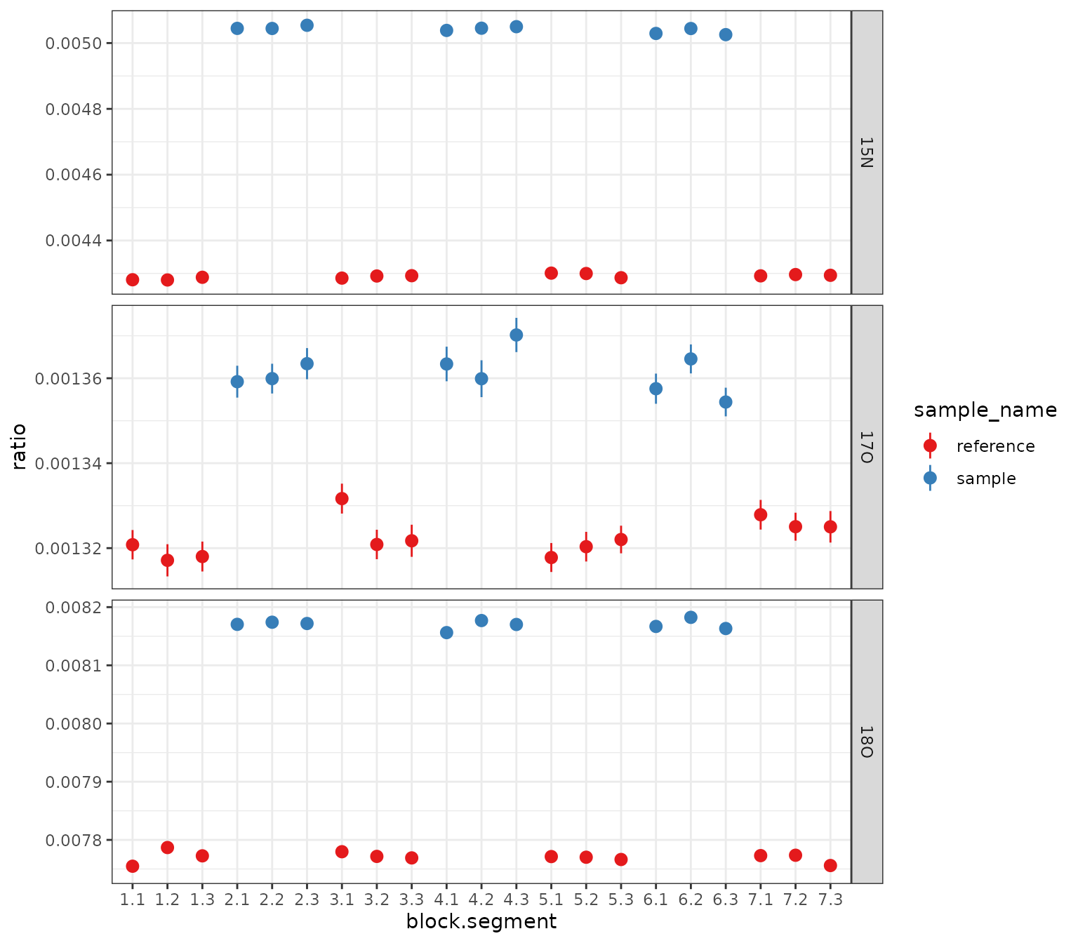
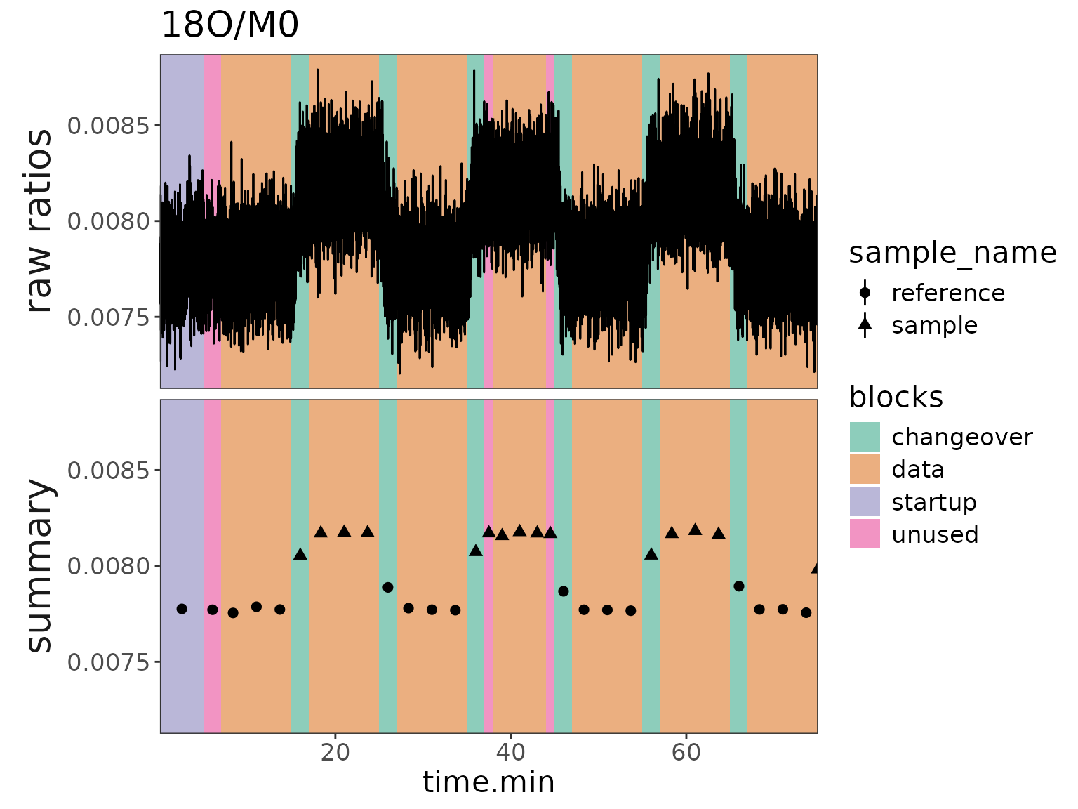
Plot 2: ratios with block backgrounds and raw data
# make a plot for 15N
plot2 <- df_w_blocks |>
  orbi_get_data(scans = everything(), peaks = everything()) |>
  filter(isotopocule == "15N") |>
  mutate(panel = "raw ratios") |>
  # raw data plot
  orbi_plot_raw_data(
    y = ratio,
    color = NULL,
    add_all_blocks = TRUE,
    show_outliers = FALSE
  ) +
   # ratio summary data
  geom_pointrange(
    data = function(df) {
      df_w_summary |>
        orbi_get_data(summary = everything()) |>
        filter(as.character(isotopocule) == df$isotopocule[1]) |>
        mutate(panel = "summary")
    },
    map = aes(
      x = mean_time.min, y = ratio,
      ymin = ratio - ratio_sem, ymax = ratio + ratio_sem,
      shape = sample_name
    ),
    size = 0.5
  ) +
  facet_grid(panel ~ ., switch = "y") +
  theme(strip.placement = "outside") +
  labs(y = NULL, title = "15N/M0")
plot2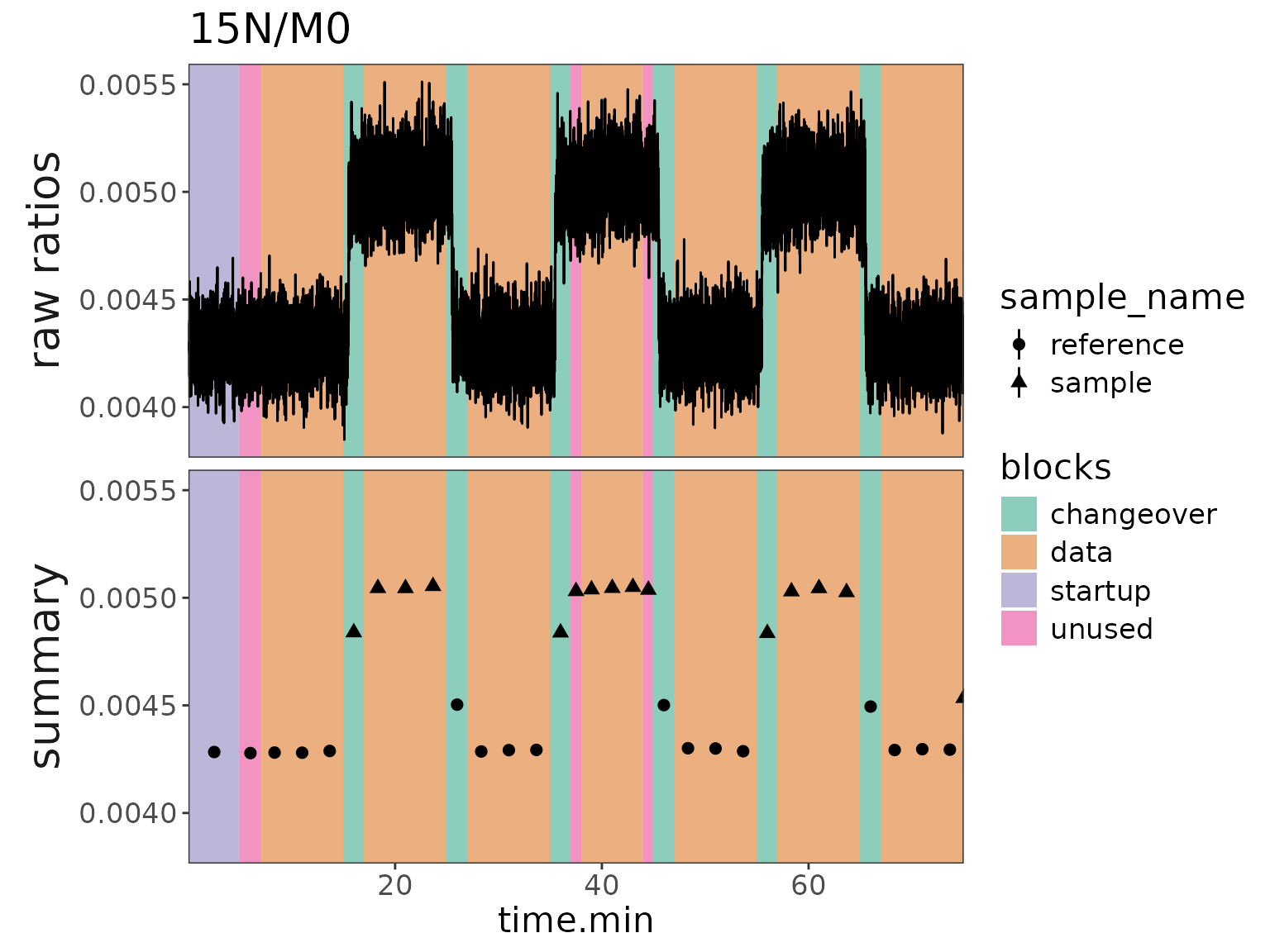
# same but with 18O
plot2 %+%
  (df_w_blocks |> orbi_get_data(scans = everything(), peaks = everything()) |>
   filter(isotopocule == "18O") |> mutate(panel = "raw ratios")) +
  labs(title = "18O/M0")